data-science – From Thread to Data

Learning Slowly: Notes on Regularization in Logistic Regression and a Small K-means Experiment

1. Learning Slowly

Over the past six weeks on Coursera, I’ve finished Google’s Course 5 Regression Analysis and am now halfway through Course 6 Machine Learning. Regression Analysis took longer than I expected, yet Machine Learning feels more basic than I initially anticipated. I’ve also decided to temporarily suspend my study of IBM’s certificate, as Google’s advanced certificate overlaps with it and covers slightly more ground.

I’ve been learning at a slower pace recently for several reasons.

I took an eleven-day vacation to Australia, followed by an additional four to five days of rest. Shortly after returning, I moved from one room to another (south-facing) at home. New furniture was bought, and a new built-in wardrobe was installed, so the whole process took a while. For all the effort, the room is super tidy and cozy now. Both Australia and my new room provide me with plenty of sunshine.

More importantly, I prefer depth over speed in my studies. That mindset inevitably slows things down. I tend to linger on topics that genuinely interest me, sometimes longer than planned.

Occasionally, a single question pulls me into a long chain of thinking. I might explore it through extended conversations, revisiting assumptions, clarifying definitions, and trying to reconcile different explanations. These detours are not always efficient, but they are often where my understanding changes most. One such detour came from learning about regularization in logistic regression. The following section is a light reflection on how my understanding evolved.

2. A Light Discussion on Logistic Regression Regularization

2.1 My First Cognition Gap – The Default Is `penalty = ‘l2’`

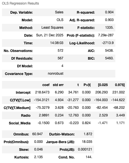
The assumptions I initially held were that statistical models always faithfully reflect mathematical definitions and fairly apply formulas unless otherwise stated. In that sense, for logistic regression, I thought the penalty was supposed to be set to none (no regularization at all) for a pure model. However, I learned incidentally through lab code that the default setting for LogisticRegression() in scikit-learn is l2, which corresponds to Ridge regularization. The lab doesn’t cover much on this topic, so I did my own research.

Unlike linear regression, where regularization isn’t set as default, logistic regression is solved by iterative optimization of the log-loss function. During this process, it may encounter the issue of separable data, where the best solution corresponds to infinite coefficients.

Data are linearly separable if there exists a vector β and an intercept β₀ such that

\beta_0 + \beta^\top x_i > 0 \quad \text{for all } y_i = 1,

\beta_0 + \beta^\top x_i < 0 \quad \text{for all } y_i = 0.

In other words, a single linear boundary can perfectly separate the two classes.

An extreme one-feature example is when, for every churned user $(y = 1), X = 1$ , whereas for all retained users $(y = 0), X = 0$ . This means that $P(y = 1 \mid X = 0) \approx 0$ and $P(y = 1 \mid X = 1) \approx 1$ .

We know that the logistic model takes the form $p = \frac{1}{1 + e^{-z}}, \quad \text{where } z = \beta_0 + \beta_1 X$ .

When $X = 0$ , we want $p \approx 0$ , which drives $\beta_0 \to -\infty$ .

When $X = 1$ , we want $p \approx 1$ , which requires $\beta_0 + \beta_1 \to +\infty$ , and therefore $\beta_1 \to +\infty$ .

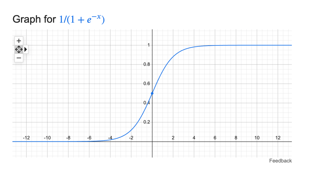
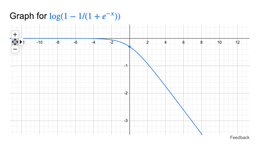
Another way of thinking about this situation is to focus on the optimization process itself. When the data are separable, once the coefficients are already near the asymptotic regions of the sigmoid, a large change in the betas only marginally improves the loss. This behavior can be seen from the shape of the sigmoid function $\pi(x) = \frac{1}{1 + e^{-x}}$ , as well as from $\log \pi(x)$ , which contributes to the loss when $y = 1$ , and $\log \bigl(1 – \pi(x)\bigr)$ which contributes when $y=0$ . The latter two terms form the log-loss.

Figures: sigmoid function

loss contribution when $y = 1$

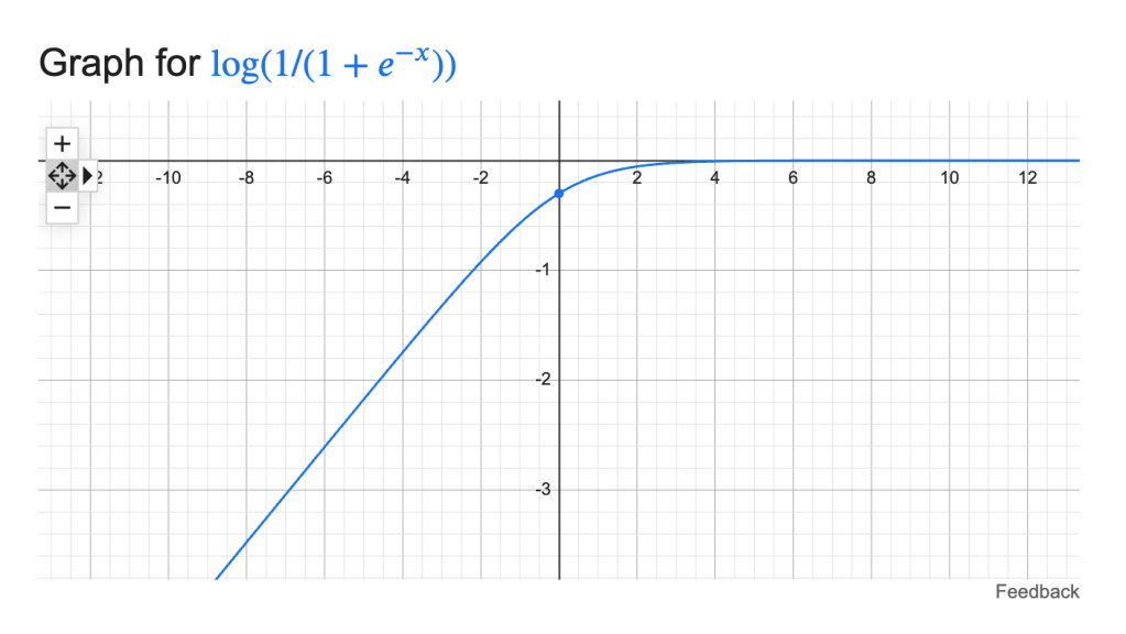
loss contribution when $y = 0$

We want to keep the betas from inflating and exploding while pushing for a better result (lower loss) during the optimization process.

Introducing a penalty to the model is like preinstalling seatbelts in a car. Large beta coefficients get penalized before they explode in the presence of separable or nearly separable data.

2.2 My Second Cognition Gap – Does the Default Penalty Parameter Make Sense?

Understanding why regularization exists naturally led me to a second question: does the default penalty parameter itself make sense?

It is always a good time to do some boring math.

For the logistic model, for each observation $i$ ,

p_i = P(y_i = 1 \mid x_i) = \frac{1}{1 + e^{-z_i}},

where

z_i = \beta_0 + \beta_1 x_{i1} + \dots + \beta_p x_{ip}.

The likelihood function over the dataset is

\mathcal{L}(\beta) = \prod_{i=1}^N p_i^{y_i} (1 – p_i)^{1 – y_i},

for binary responses $y_i \in \{0,1\}$ .

Taking the negative log leads to the loss for a single observation,

\ell_i(\beta) = – y_i \log(p_i) – (1 – y_i)\log(1 – p_i).

The loss over the entire dataset, which scikit-learn uses in its mean form, is

J(\beta) = \frac{1}{N} \sum_{i=1}^N \ell_i(\beta).

When adding L2 regularization, the objective becomes the log-loss plus a penalty term:

J(\beta) = \frac{1}{N} \sum_{i=1}^N \ell_i(\beta) \;+\; \frac{1}{2CN} \sum_{j=1}^p \beta_j^2,

where $C$ is the inverse regularization strength. In scikit-learn, the default value of $C$ is 1.

While I was initially picking up this concept, the formula ChatGPT originally provided to me missed the $1/N$ factor in the penalty term, which made the penalty appear excessively large. As a result, the penalty and the original loss looked completely out of proportion, and the regularization term seemed arbitrary and dominating. This confused me for quite some time. I spent hours discussing this with GPT, trying to make sense of the formula, until we eventually realized that the original expression was incorrect! (I just wanted to scream at that point — and I probably did.)

After correcting the formula by including the proper $1/N$ scaling, the default parameter choice $C=1$ started to make sense. It is reasonable and tolerant enough not to hinder overall model performance on generally good data. By “good data,” I mean data with no (near) separation, no extreme multicollinearity, sufficient sample size relative to the number of features, and coefficients that are stable across resamples.

When the data are good, logistic regression with Ridge and without Ridge produces almost identical results. The regularization term quietly disappears. Regularization mainly matters when the unregularized solution is unstable. In that sense, it really behaves like a seatbelt: always present, but only noticeable when something goes wrong. This behavior differs from Ridge in linear regression, where coefficient shrinkage is present even when the data are well behaved.

I also learned that the parameter $C$ often requires tuning in special cases, and this tuning is typically performed on a logarithmic scale (for example, $C = 0.1 \rightarrow 1 \rightarrow 10$ ).

Finally, it is worth noting that, in practice, we almost always apply StandardScaler() before fitting the model. Since the scale of the coefficients directly affects the penalty, unscaled features can lead to coefficients being penalized unevenly. For example, without standardization, features with smaller scales may be penalized more heavily because they require larger coefficients.

3. A Small K-means Color Quantization Experiment

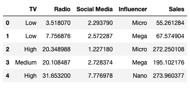
Not all learning moments need to be heavy. As another part of my recent study, I experimented with k-means clustering through a simple color quantization project, which I found quite interesting. In this exercise, we ignore the spatial position of each pixel in the image and group pixels into $k$ representative colors based on their RGB values. Each pixel is then replaced by its cluster’s representative color to approximate the original image.

Below are my current profile picture (taken in Australia), the centroid colors learned by k-means (ordered by brightness) with $k = 9$ , and the corresponding quantized image (yes, it comprises only 9 colors).

Figures: Centroid colors

Original image and quantized image

For now, this is where my understanding stands.

A Case Study of Application on the Variance Inflation Factor (VIF) in Multiple Linear Regression

0. Why This Case Matters

This article examines a reference solution provided in a lab activity, using it as a case study to illustrate a common pitfall in the use of Variance Inflation Factor (VIF): treating it as a standalone decision rule rather than a diagnostic tool to be interpreted in the context of the full regression model. By examining competing model specifications side by side, this case illustrates why variable selection should be guided by marginal explanatory power, not VIF thresholds alone.

The case and data are drawn from the lab activity ‘Perform Multiple Linear Regression’ in Module 3 of Course 5, Regression analysis: Simplify Complex Data Relationships, from the Google Advanced Data Analytics Professional Certificate on Coursera. The data originate from a Kaggle dataset (https://www.kaggle.com/datasets/harrimansaragih/dummy-advertising-and-sales-data) and have been modified for instructional purposes in this course.

1. General Introduction to the Case

In this case study, we analyze a small business’ historical marketing promotion data. Each row corresponds to an individual marketing promotion in which the business uses TV, social media, radio and influencer campaigns to increase sales. The goal is to conduct a multiple linear regression analysis to estimate sales from a combination of independent variables.

Following the exemplar, the dataset is read using pandas and stored as data. The output of data.head() is shown below:

The features in the data are:

TV: television promotion budget (Low, Medium, or High)
Radio: radio promotion budget (in millions of dollars)
Social Media: social media promotion budget (in millions of dollars)
Influencer: type of influencer the promotion collaborated with (Mega, Macro, Nano or Micro)
Sales: total of sales (in millions of dollars)

A pair plot is shown below:

From the plot, we can see that both Social Media and Radio are positively correlated with Sales. If only one were to be selected, Radio appears to be a stronger indicator than Social Media, as the points cluster more closely around the fitted line. Thus, either Radio alone or the combination of Radio and Social Media could plausibly be selected as independent variables.

The mean Sales for each category in TV and for each category in Influencer are:

There is substantial variation in mean sales across the categories of TV, while mean sales vary very little across Influencer categories. The result indicates that TV should be retained as an independent variable, while Influencer can reasonably be discarded.

As the ols() function in Python doesn’t accept variable names containing spaces, we rename Social Media to Social_Media.

Based on the analysis above, our task is to choose between the following two models:

Sales ~ C(TV) + Radio + Social_Media
Sales ~ C(TV) + Radio

2. The Pitfall in the Use of Variance Inflation Factor (VIF)

For the succeeding sections, assume we have imported the following libraries in Python:

import pandas as pd
import statsmodels.api as sm
from patsy import dmatrices
from statsmodels.stats.outliers_influence import variance_inflation_factor

The exemplar then fits the OLS model of Sales ~ C(TV) + Radio, tests the model assumptions of linearity, residual normality, and homoscedasticity, which are methodologically sound applications.

However, the method by which the exemplar checks the no multicollinearity assumption is worth reexamining.

The exemplar runs the following code to compute the VIF values for Radio and Social_Media:

x = data[['Radio','Social_Media']]
vif = [variance_inflation_factor(x.values, i) for i in range(x.shape[1])]
df_vif = pd.DataFrame(vif, index = x.columns, columns = ['VIF'])
df_vif

The exemplar concludes that the VIF when both Radio and Social_Media are included in the model is 5.17 for each variable, indicating high multicollinearity.

By revisiting the method, we find that the exemplar’s application leads quickly to the conclusion that Social_Media should be excluded due to multicollinearity, without comparing alternative model specifications.

To understand why this matters, it is useful to briefly revisit what VIF measures. The variance inflation factor (VIF) is one of the most widely used diagnostics for multicollinearity, largely due to its simplicity and broad applicability. It quantifies how much the variance (and thus uncertainty) of a regression coefficient increases due to multicollinearity among predictors, relative to a model in which the predictors are independent. Higher VIF values indicate less stable coefficient estimates that are more sensitive to small changes in the data.

For a given predictor $X_j$ , the VIF is defined as

\text{VIF}_j = \frac{1}{1 – R_j^2}

where $R_j^2$ is obtained by regressing $X_j$ on all other predictors in the model.

In practice, VIF values are commonly interpreted using the following suggestive (rather than definitive) thresholds: a VIF of 1 indicates no multicollinearity; values between 1 and 5 suggest mild and typically acceptable multicollinearity; values between 5 and 10 indicate moderate and potentially concerning multicollinearity; and values greater than 10 are often taken as evidence of severe multicollinearity.

A more robust application in this case consists of the following steps:

Computing VIF with an intercept
Using the same design matrix as the regression model, including the categorical variable TV
Evaluating alternative model specifications to assess the marginal contribution of Social_Media

Let’s begin with the reasoning behind step 1: Add intercept to calculate VIF. VIF measures how well one column can be explained by the other columns in the design matrix. When we omit the constant (intercept), we force every auxiliary regression to go through the origin. That changes the $R^2$ . What the statsmodels internally run is $\text{Radio} = \beta \cdot \text{Social\_Media}$ (no intercept), whereas we actually want the model to be $\text{Radio} = \beta_0 + \beta \cdot \text{Social\_Media}$ . That’s why we need to update the code to include the intercept:

x = data[['Radio','Social_Media']]
x = sm.add_constant(x)
vif = [variance_inflation_factor(x.values, i) for i in range(x.shape[1])]
df_vif = pd.DataFrame(vif, index = x.columns, columns = ['VIF'])
df_vif

This gives us the result:

The result aligns more closely with the correct analytical interpretation than the previous one.

However, this is not sufficient on its own. By definition, VIF should be computed using the same design matrix as the regression model including the intercept, because multicollinearity is a group-level phenomenon. Multicollinearity is not about any single pair of variables. It is about near-linear dependence among a set of predictors. As we’ve decided to include categorical variable TV into the model, we should use the same design matrix in the code. A modified code could be:

y, X = dmatrices('Sales ~ C(TV) + Radio + Social_Media',data,return_type='dataframe')
vif = [variance_inflation_factor(X.values, i) for i in range(X.shape[1])]
df_vif = pd.DataFrame(vif, index = X.columns, columns = ['VIF'])
df_vif

patsy’s dmatrices adds the intercept. It also returns the same encoded TV dummies aligned with statsmodels, because statsmodels internally uses patsy. The full design matrix of the right-hand side of the formula is saved in X. The code returns the result:

Once VIF is computed on the full regression design matrix, VIF for Radio is 3.46, for Social_Media 1.66, and for TV dummies below common concern threshold (we should always ignore intercept’s VIF in our interpretation), suggesting no problematic multicollinearity.

To determine whether Social_Media should be excluded as an independent variable, we compare the model summaries from two specifications:

A. Model without Social_Media:

B. Model with Social_Media:

We can see that Model A exhibits strong overall fit, with all coefficients statistically significant, an adjusted $R^2$ of 0.904, and a highly significant F-statistic. Model B doesn’t seem to be an improvement from A, with Social_Media’s p value of 0.824, and Adjusted $R^2$ of 0.903 which is slightly worse than Model A’s. Per model results, we can now safely drop Social_Media.

Based on the analysis above, unlike the exemplar’s conclusion, we are not dropping Social_Media because of multicollinearity. We are dropping it because it adds no marginal explanatory power once Radio and TV are already in the model. The lack of significance is due to redundancy, not problematic multicollinearity.

Through this case study, working on these steps helped clarify several common misconceptions and led to three key principles for interpreting VIF, which are discussed in the following sections.

3. Principle 1: High correlation does not automatically imply multicollinearity

Multicollinearity refers to a situation in which one or more predictors in a regression model can be well approximated by a linear combination of the others.

For now, consider the simplified case of two predictors.

Examining standard (suggestive rather than definitive) VIF interpretation guidelines, one may notice that the threshold for diagnosing multicollinearity in the two-predictor case appears unusually strict. When only two predictors are present, the correlation coefficient must exceed approximately 0.9 before VIF reaches a value of 5, a value that is commonly used to flag potential multicollinearity. This is because, with two predictors, the squared correlation coefficient is equivalent to the $R^2$ obtained by regressing one predictor on the other. Substituting this into the VIF formula, $\text{VIF} = \frac{1}{1 – r^2}$ , yields a value of approximately 5 when r=0.9.

By contrast, although there is no universal cutoff for “high” correlation, values above 0.6 are often considered strong and are visually apparent in scatter plots. However, when r=0.6, the corresponding VIF is only about 1.56, which is well below commonly used thresholds for concern.

Following is a scatter plot of two variables with a correlation coefficient of 0.63, corresponding to a VIF of approximately 1.66:

The key intuition linking these observations is that even at moderately high correlation levels, a substantial portion of variation remains unexplained. For example, when r=0.6, roughly 64% of the variance is unexplained, and even when r=0.8, about 36% remains unexplained. In such cases, an additional predictor can still provide meaningful marginal explanatory power, which is why high correlation alone does not imply problematic multicollinearity under a rigorous definition.

Notably, as the correlation coefficient approaches 1, VIF increases rapidly and nonlinearly. While the two-predictor case requires extremely high correlation to trigger concern, the presence of additional predictors changes this dynamic. With multiple predictors, even moderate pairwise correlations can inflate VIF. For this reason, all predictors should be included when computing VIF to ensure that the diagnostic reflects the full regression design.

4. Principle 2: Multicollinearity does not imply high pairwise correlation

Correlation is fundamentally a bivariate concept. When discussing correlation among multiple variables, we are typically referring to pairwise correlations between variable pairs.

It is possible to construct a case where pairwise correlations are low or even zero, yet multicollinearity is present.

Consider the constructed example $X_5 = X_1 + X_2 + X_3 + X_4 +\epsilon$ , where $X_1$ , $X_2$ , $X_3$ , and $X_4$ are mutually uncorrelated, and $\epsilon$ is a noise term independent of the other predictors. By construction, pairwise correlations between predictors can be small, including those involving $X_5$ . Intuitively, the noise term increases the overall variability of $X_5$ without increasing its shared variation with any single predictor, allowing pairwise correlations to remain small. However, when considered jointly, $X_5$ can still be well explained by a linear combination of $X_1$ , $X_2$ , $X_3$ and $X_4$ , resulting in strong multicollinearity in a regression model of the form $Y = aX_1 + bX_2 + cX_3 + dX_4 + eX_5 + intercept$ .

This example illustrates that multicollinearity does not imply high pairwise correlation. Consequently, multicollinearity should be assessed using the full regression model, rather than inferred from pairwise correlations alone.

5. Principle 3: A higher VIF does not imply that a variable should be dropped

This case study clarifies a common misunderstanding in the interpretation of VIF. VIF values should not be compared mechanically across predictors to determine which variable to remove from a regression model.

Multicollinearity is a group-level issue among predictors: removing any one of the collinear variables can restore model stability, and the final choice should be based on each variable’s marginal contribution to explaining the response. In other words, VIF diagnoses group instability, not variable importance.

The marketing case discussed above illustrates this clearly. Although the VIF for Radio (3.46) is higher than that for Social_Media (1.66), Social_Media is the variable that is removed from the model. This shows that variable selection should be guided by marginal explanatory power rather than by relative VIF values alone.

In predictive modeling contexts, where the primary goal is generalization rather than coefficient interpretability, multicollinearity is often addressed through regularization techniques—such as Ridge, Lasso, and Elastic Net—rather than explicit variable removal. However, since the focus of this discussion is the interpretation and application of VIF, these models will not be explored in detail here.

6. Conclusion

This case study illustrates that multicollinearity is fundamentally a group-level phenomenon and cannot be reliably inferred from pairwise correlations alone. VIF serves as a diagnostic tool for assessing instability among predictors within a specified regression model, which is why it must be computed using the full design matrix, including the intercept. However, diagnosing multicollinearity is only one step in model building. Decisions about whether to retain or remove predictors should ultimately be guided by their marginal contribution to explaining the response, rather than by VIF values in isolation. Used in this way, VIF supports sound modeling decisions rather than replacing them.